R을 이용한 이동평균선 일봉챠트에 같이 그리기

주식 책 보면 가장 먼저 나오는 종가 이동 평균 선을 일봉챠트에 그리는 R 코드입니다.

이동평균 구하는 방법도 다양한데요 그중 4가지 정도에 대해서 챠트를 그려 보겠습니다.

1. 단순이동평균 : SMA, calculates the arithmetic mean of the series over the past n observations.

우리가 흔히 알고 있는 바로 그것입니다.

2. 지수평활법 : EMA, calculates an exponentially-weighted mean, giving more weight to recent observations. See Warning section below.

최근 가격에 더 가중치를 두고 계산하는 방법입니다.가중치는 0과 1사이의 값입니다

3. 선형가중이동평균 : WMA is similar to an EMA, but with linear weighting if the length of wts is equal to n. If the length of wts is equal to the length of x, the WMA will use the values of wts as weights.

역시 최근 가격에 가중치를 주고 계산합니다.

4. 거래량가중이동평균 : VWAP calculate the volume-weighted moving average price.

거래량에 따라 가중치를 주어 계산하는 방법입니다.

 # plotly 챠트 library(plotly) library(quantmod) samsung <- getSymbols('005930.KS', auto.assign = FALSE) colnames(samsung) <- c('open','high','low','close','volume','adjusted') #samsung$rtn <- ROC(Cl(samsung)) #일일 수익률 samsung <- na.omit(samsung) # NA 제거 # basic example of ohlc charts df <- data.frame(Date=index(samsung),coredata(samsung)) df <- tail(df, 600) # cutom colors i <- list(line = list(color = 'red')) d <- list(line = list(color = 'blue')) fig <- df %>% plot_ly(x = ~Date, type="candlestick", open = ~open, close = ~close, high = ~high, low = ~low, increasing = i, decreasing = d) fig <- fig %>% add_lines(x = ~Date, y = ~close, line = list(color = 'black', width = 2), inherit = F) fig <- fig %>% layout(title = "Basic Candlestick Chart", xaxis = list(rangeslider = list(visible = F)), showlegend = FALSE) fig # 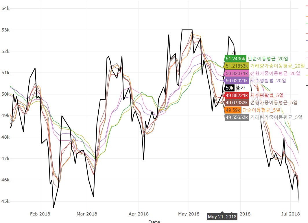이동평균 추가 df <- data.frame(Date=index(samsung),coredata(samsung)) # 단순이동평균 SMA : calculates the arithmetic mean of the series over the past n observations. df$MA5 <- SMA(df$close,n=5) df$MA20 <- SMA(df$close,n=20) # 지수평활법 EMA : calculates an exponentially-weighted mean, giving more weight to recent observations. See Warning section below. df$EMA5 <- EMA(df$close,n=5) df$EMA20 <- EMA(df$close,n=20) # 선형가중이동평균 WMA is similar to an EMA, but with linear weighting if the length of wts is equal to n. If the length of wts is equal to the length of x, the WMA will use the values of wts as weights. df$WMA5 <- WMA(df$close,n=5) df$WMA20 <- WMA(df$close,n=20) # 거래량가중이동평균 VWAP calculate the volume-weighted moving average price. df$VWAP5 <- VWAP(df$close,df$volume,n=5) df$VWAP20 <- VWAP(df$close,df$volume,n=20) df <- tail(df, 300) i <- list(line = list(color = 'red')) d <- list(line = list(color = 'blue')) fig <- df %>% plot_ly(x = ~Date, type="candlestick", name = "일봉", open = ~open, close = ~close, high = ~high, low = ~low, increasing = i, decreasing = d) fig <- fig %>% add_lines(x = ~Date, y = ~MA5 , name = "단순이동평균_5일", line = list( width = 1), legendgroup = "SMA",inherit = F) fig <- fig %>% add_lines(x = ~Date, y = ~MA20 , name = "단순이동평균_20일", line = list( width = 1), legendgroup = "SMA",inherit = F) fig <- fig %>% add_lines(x = ~Date, y = ~EMA5 , name = "지수평활법_5일", line = list( width = 1), legendgroup = "EMA",inherit = F) fig <- fig %>% add_lines(x = ~Date, y = ~EMA20 , name = "지수평활법_20일", line = list( width = 1), legendgroup = "EMA",inherit = F) fig <- fig %>% add_lines(x = ~Date, y = ~WMA5 , name = "선형가중이동평균_5일", line = list( width = 1), legendgroup = "WMA",inherit = F) fig <- fig %>% add_lines(x = ~Date, y = ~WMA20 , name = "선형가중이동평균_20일", line = list( width = 1), legendgroup = "WMA",inherit = F) fig <- fig %>% add_lines(x = ~Date, y = ~VWAP5 , name = "거래량가중이동평균_5일", line = list( width = 1), legendgroup = "VWAP",inherit = F) fig <- fig %>% add_lines(x = ~Date, y = ~VWAP20 , name = "거래량가중이동평균_20일", line = list( width = 1), legendgroup = "VWAP",inherit = F) fig <- fig %>% add_lines(x = ~Date, y = ~close, name='종가', line = list(color = 'black', width = 2), inherit = F) fig <- fig %>% layout(title = "Basic Candlestick Chart", xaxis = list(rangeslider = list(visible = F)), showlegend = TRUE) fig